Lecture 2 Notes: MIT Linear Algebra (18.06) [Elimination with Matrices]

Elimination with Matrices

Important point: A matrix times a column is a column, a matrix times a row is a row

Given the following equations, solve for x, y, and z using elimination and back substitution:

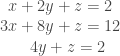
We start by forming our matrix, leaving out the right side of the equations.

Elimination (success/failure)

Using elimination, our goal is to turn our original matrix into one that looks like this where n represents some arbitrary number:

To get to this destination we:
– go row by row
– keep the first row
– determine what number multiplied to the row above when subtracted
by the current row will get us closer our destination matrix

Step by step, here are what the matrices will look like

Let’s start with our original matrix.

We keep the first row, so we take a look at the second row. We ask ourselves: What must I do to the first row ([1, 2, 1]) such that when subtracted by the second row ([3, 8, 1]), the first number is a zero? Our aim is to get a row that look like this ([0, n, n], again n being any arbitrary number). The answer is that we must multiply the first row by 3, which will give us [3, 6, 3]. We then subtract this by the second row to give us [0, 2, -2]. We now work with this new matrix when going to the third row.

We repeat this step for our new matrix.

We have to get a row that looks like [0, 0, n]. As we can see, we’re already halfway there since we were given the first 0 to begin with. Same process for the other 0: what must I do to the row above ([0, 2, 2]) such that when subtracted by the third row ([0, 4, 1]) the first two numbers are zero? Similar to the process above, we must multiply the second row by 2, which will give us [0, 4, -4]. We then subtract this by the third row to give us [0, 0, 5]. Now, we have our final matrix.

Pivot numbers

The diagonal line of numbers starting from the top-left (1, 2, 5) are called pivot numbers. An important note is that if any of these numbers were zero to start with, we would have to switch rows around and try again.

Right hand side

Notice we haven’t touched the right side of the equations yet, but that’s an easy step to do afterwards. This is also the way software solves systems of equations.

Let’s take our matrices we solved through and let’s augment them by including the numbers from the right hand side of the equations. These matrices are known as augmented matrices.

You get the new fourth column by following a similar process of taking the multiplier, multiply the number above the row in question and subtracting the current row number by that value.

For example, the number we multiplied the first row in the un-augmented matrices was a 3. We start in the second row and multiply the 2 in the first by 3 to make 6. Subtract the 12 in the second row by the 6 and we get 6, which is our new second row value.

Back Substitution

Our new equations are:

Very simple from this point, start with the last equation and move up, solving for a variable at a time. The solutions turns out to be: z = -2, y = 1, x = 2.

Elimination Matrices

Let’s use the first and second matrices of our un-augmented matrices as an example. What matrix do I multiply the first matrix by to get the second matrix? How do I subtract 3x from row 1 from row 2?

We’ll start with the identity matrix which when multiplied by some matrix, gives you back that same matrix. We need to fix this so that we have 3 of row 1 subtracted from row 2. Here is the solution.

Matrix Multiplication

Important point: Matrices are noncommutative, so order matters!

How to switch rows of a matrix

Inverses

How to undo elimination: Simply switch a sign to get back to the identity matrix